こんにちは。
その1でラッソの概要と大きな特徴であるスパース性を確認しました。
今回からはラッソ実装に向けて数学を頑張りましょう。
Notationのについて
- Obj (objective function)
- OLS (Ordinary least squares) (回帰の残差平方和)
 : データ数
 : 次元(特徴)
 :
:  番目の特徴
番目の特徴
 :
:  番目の観測データ
 のうちに対応するもの
目的関数について
今回、つまりラッソの目的関数は以下の通り
![\[Obj(\theta) & = OLS(\theta) + \lambda | \theta |_1^1\]](https://research.miidas.jp/wp-content/ql-cache/quicklatex.com-7e0d681388f2a356aaf5206690b1a4e1_l3.png "Rendered by QuickLaTeX.com")
![\[= \frac{1}{2} \sum_{i=1}^m \left[y^{(i)} - \sum_{j=0}^n \theta_j x_j^{(i)}\right]^2 + \lambda \sum_{j=0}^n |\theta_j|\]](https://research.miidas.jp/wp-content/ql-cache/quicklatex.com-d3c0281cbd2637a8dbe9ff04a0f1fcc6_l3.png "Rendered by QuickLaTeX.com")
(OLS)の勾配について
上の目的関数は微分できません。なのでひとまず置いておいて
OLSをいつも通り微分して微分を計算します。
後々のため、今回は勾配でなく、での微分を計算します。
![\[\frac{\partial }{\partial \theta_j} OLS(\theta) & = - \sum_{i=1}^m x_j^{(i)} \left[y^{(i)} - \sum_{j=0}^n \theta_j x_j^{(i)}\right]\]](https://research.miidas.jp/wp-content/ql-cache/quicklatex.com-a64d5d20e76233a2098cab78e929ca24_l3.png "Rendered by QuickLaTeX.com")
![\[= - \sum_{i=1}^m x_j^{(i)} \left[y^{(i)} - \sum_{k \neq j}^n \theta_k x_k^{(i)} - \theta_j x_j^{(i)}\right]\]](https://research.miidas.jp/wp-content/ql-cache/quicklatex.com-77c0eb5aab2b2dd74afc2122036d8abd_l3.png "Rendered by QuickLaTeX.com")
![\[= - \sum_{i=1}^m x_j^{(i)} \left[y^{(i)} - \sum_{k \neq j}^n \theta_k x_k^{(i)} \right] + \theta_j \sum_{i=1}^m (x_j^{(i)})^2\]](https://research.miidas.jp/wp-content/ql-cache/quicklatex.com-26652c614728dad57bf0147da24f8045_l3.png "Rendered by QuickLaTeX.com")
簡単のためこれを次のように表します。
![\[:= - \rho_j + \theta_j z_j\]](https://research.miidas.jp/wp-content/ql-cache/quicklatex.com-1c6e98babc4b2d551012b228ff032e28_l3.png "Rendered by QuickLaTeX.com")
L1-normの微分について
 -normは微分できないとわかりました。なので
微分できるように、微分という概念を拡張します。そこで出てくるのが
です。wikiのリンク
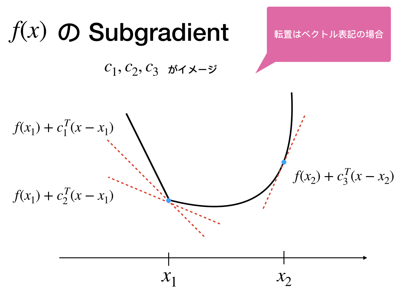
定義(劣微分)
Convex  の点
の点  における劣微分は次の条件を満たす
  で定義する。
(簡単のため についてはなし、微分の代わりに勾配という言葉を使っている)
![\[\frac{\partial f }{\partial x}\bigg |<em>{x=x_0} = { c \in \mathbb{R} : f(x) \geq f(x_0) + c(x - x_0) , \forall x \in I }\]](https://research.miidas.jp/wp-content/ql-cache/quicklatex.com-789e8c3b5086bbb401a79e79728ae6d2_l3.png "Rendered by QuickLaTeX.com")
書き換えると
における劣勾配は次の閉区間の集合である。
![\[a = \lim</em>{x \rightarrow -x_0} \frac{f((x) - f(x_0)}{x - x_0}\]](https://research.miidas.jp/wp-content/ql-cache/quicklatex.com-f5e3d0f90e01a0aefd7ea0183bb5a56c_l3.png "Rendered by QuickLaTeX.com")
![\[b = \lim_{x \rightarrow +x_0} \frac{f((x) - f(x_0)}{x - x_0}\]](https://research.miidas.jp/wp-content/ql-cache/quicklatex.com-decfa1785ee39ab9c560920400e55a0c_l3.png "Rendered by QuickLaTeX.com")
![\[\frac{\partial f }{\partial x}\bigg |_{x=x_0} = [a,b]\]](https://research.miidas.jp/wp-content/ql-cache/quicklatex.com-aa05afe0345250b555c0dabf52c4c87c_l3.png "Rendered by QuickLaTeX.com")
これが勾配の拡張になっていることは微分可能な点においてその劣勾配が一点集合になることからわかる
実はこれは簡単で、場合分けして綺麗に微分できるところの間を1つの微分の集合と見るのです。
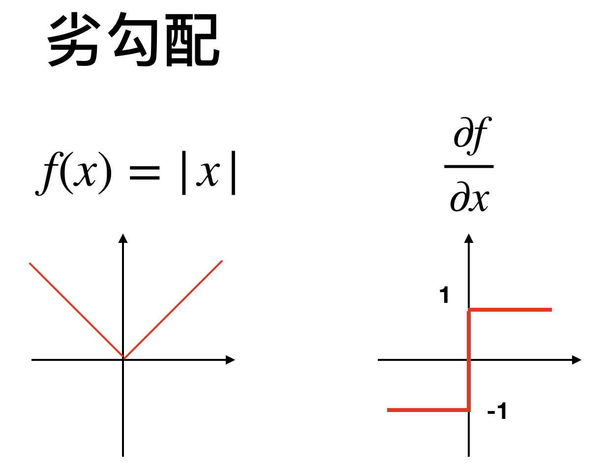
今回のノルム、つまり
![\[f(x) = |x|\]](https://research.miidas.jp/wp-content/ql-cache/quicklatex.com-c8294584bc63ed979ae6270e3e56b819_l3.png "Rendered by QuickLaTeX.com")
を例にとると、
(1) 
(2) 
そしてこの間の集合を0での微分とするのが劣勾配
(3) ![\begin{align*} \texttt{if } x = 0 ~~ , ~~ \frac{\partial f}{\partial x} = [-1,1] \end{align*}](https://research.miidas.jp/wp-content/ql-cache/quicklatex.com-e27061f1c07b8d8c8407dc099cd4e9c5_l3.png "Rendered by QuickLaTeX.com")
次のはイメージ図
ではこの劣勾配を使って今回の目的関数の第2項を微分してゼロとおきます。
(4) 
(5) 
ここで先ほどと同様に場合分けを行って
(6) 
(7) 
そして、
(8) ![\begin{align*} \texttt{if } \theta_j = 0 ~~ , ~~ 0 = [-\rho_j - \lambda ,-\rho_j + \lambda ] \end{align*}](https://research.miidas.jp/wp-content/ql-cache/quicklatex.com-9d03979fa9200a3ba1e07947d88550f1_l3.png "Rendered by QuickLaTeX.com")
ですね。文字が多くなってしまったので再確認ですが、目標はを求めることです。上の2つの式は簡単に求まりますが、3つ目の式については閉区間に0が含まれるという条件で考えましょう。なので
(9) ![\begin{align*} 0 \in [-\rho_j - \lambda ,-\rho_j + \lambda ] \end{align*}](https://research.miidas.jp/wp-content/ql-cache/quicklatex.com-67afd552e9a39fe305ff82e521eb9ebb_l3.png "Rendered by QuickLaTeX.com")
(10) 
(11) 
なので
(12) 
まとめると
(13) 
(14) 
(15) 
となります。ちなみにこの場合分けからSoft thresholding functionという関数が定義されます。
最後に劣微分と一緒にplotを見てみましょう。
微分できなくてよく使う関数をたまたま思い出しました。ニューラルネットワークで使うRELU fucntionですね。
– 活性化関数ReLUとその類似関数
他にも色々あるようです。
色々計算づくしでしたが微分を計算できました。あとは最適化のみですが今までは勾配法を使っていましたが「微分不可能な場合は勾配法は無理」なので他の最適化法が必要です。そこでLassoの問題ではいくつかのメジャーな方法があります。
- Coordinate descent(座標降下法)
- ISTA (メジャライザー最小化)
- FISTA (高速化)
です。もっとも簡単なのは座標降下法です。メジャライザーはテイラー展開を用いて上界を扱うものですがこれらについては次回解説します。
でわ。