こんにちは。いまだにたまに暑いと感じるkzです。今回はなにをやりましょうかねえ。
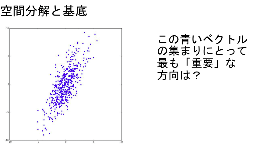
このデータは見ての通り2次元(平面)データです。これを1次元(直線)に置き換えたいです。
各点の配置は?
置き換える時に重要なのは距離感です。離れていた点通しが置き換えた先でご近所さんになると元のデータをうまく表現できてるとは言えませんよね。それが次の図です。
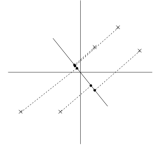
離れていたはずがご近所さんになってしまっています。一方で次の図はどうでしょう、
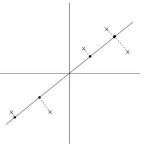 さっきよりはうまく元のデータを表せていますよね。ではこれを先ほどの青いデータで考えると
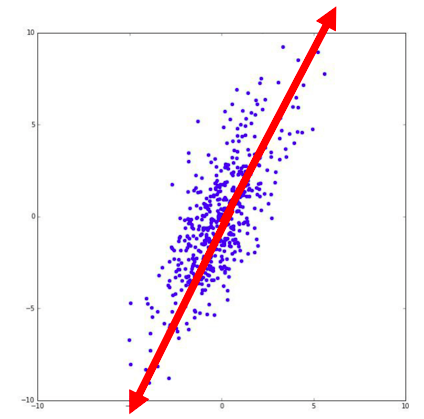
この赤矢印上に先ほどと同様にして点を置き換えれば つまり2次元のデータを1次元で説明できることになります。
では本日の本題に入りましょう。
上の赤矢印(軸)
どうやっていい軸を選びましょうか。じーっと見てみましょう。広がっている方向に矢印が伸びていますね。つまりいい軸とはデータを矢印だけで表現したものと捉えることができそうです。では具体的にいい軸(ベクトル)をどう求めるかを考えましょう。
とりえあず求めるベクトルを とします。今長さは別に興味ないので
 とします。
とします。
正射影ベクトルを考えます。下の緑( )はaのbへの射影です。
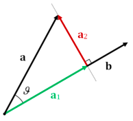
上の図は をデータ点
をデータ点 を求めたいベクトルとした時に
 の最小化もしくわの最大化がしたいことになります。この事実は次のgifより明らかです。
なので今回はデータを 、ベクトルをとするとその正射影ベクトルは
![\[ \frac{x_i \cdot v}{|v|} v\]](https://research.miidas.jp/wp-content/ql-cache/quicklatex.com-de970521584d6f0d90ad134959157c54_l3.png "Rendered by QuickLaTeX.com")
です。これを全データで最大化したいので次のようになります。 は都合上のものです!
![\[\frac{1}{N-1} \sum_{i=1}^{N} (x_i^T v)^2 = \frac{1}{N-1} \sum_{i=1}^{N} (x_i^T v)^T(x_i^T v)\]](https://research.miidas.jp/wp-content/ql-cache/quicklatex.com-acdb94ec8ba931d0a6fdf333756dfcae_l3.png "Rendered by QuickLaTeX.com")
![\[= v^T \left(\frac{1}{N-1}\sum_{i=1}^{N} ( x_i x_i^T)\right) v\]](https://research.miidas.jp/wp-content/ql-cache/quicklatex.com-30106ea2ed1ea3f9cc4c4964f174e1b2_l3.png "Rendered by QuickLaTeX.com")
となります。 これって何でしょう?一応ですが
 は共に縦ベクトルです。
そうです共分散行列です。これを と書くことにします。すると
![\[v^T \Sigma v \]](https://research.miidas.jp/wp-content/ql-cache/quicklatex.com-04b8c60263a94b350ec7b4939197308a_l3.png "Rendered by QuickLaTeX.com")
が今回の目的関数です。今まで通りならこれを最大化するだけだったんですが今回は制約があります。
![\[| v | = 1 \]](https://research.miidas.jp/wp-content/ql-cache/quicklatex.com-d2c7294ea5e286872d590e7bded80368_l3.png "Rendered by QuickLaTeX.com")
です。この状況を条件付き極値問題と言います。これを解くには技が必要です。
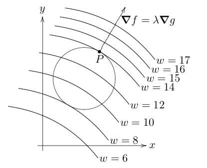
![\[\texttt{Maximize} ~~~ f(x,y) \]](https://research.miidas.jp/wp-content/ql-cache/quicklatex.com-58813bd583dc0e4e927ad0e0bb770683_l3.png "Rendered by QuickLaTeX.com")
![\[\texttt{Subject to} ~~~ g(x,y)=0 \]](https://research.miidas.jp/wp-content/ql-cache/quicklatex.com-dc13a656c5f838bd8e77fae427f93719_l3.png "Rendered by QuickLaTeX.com")
を考える、 が
が 級(微分可能かつ導関数が連続)とする。点Pが極値をとるならば
![\[\mathcal{L} (x,y, \lambda) = f(x,y) - \lambda g(x,y) \]](https://research.miidas.jp/wp-content/ql-cache/quicklatex.com-6046d51760ee5382193d6119b82860ac_l3.png "Rendered by QuickLaTeX.com")
![\[\nabla f (P) - \lambda \nabla g(P) = 0\]](https://research.miidas.jp/wp-content/ql-cache/quicklatex.com-11b0b2ef58f25c09245b2cd33abf8ea5_l3.png "Rendered by QuickLaTeX.com")
を満たす。あくまで候補点です。要点だけいうと勾配が平行になる点です。
 証明や詳しい解説はここにあります。
- https://en.wikipedia.org/wiki/Lagrange_multiplier
- http://www.yunabe.jp/docs/lagrange_multiplier.html
- https://ocw.mit.edu/courses/mathematics/18-02sc-multivariable-calculus-fall-2010/2.-partial-derivatives/part-c-lagrange-multipliers-and-constrained-differentials/session-40-proof-of-lagrange-multipliers/MIT18_02SC_notes_22.pdf
これをラグランジュの未定乗数法と言います。これを使って計算しましょう。
![\[ \mathcal{L} (v, \lambda) = v^T\Sigma v - \lambda (| v|)\]](https://research.miidas.jp/wp-content/ql-cache/quicklatex.com-0114f16c496bb0dd9a42c9c64754700b_l3.png "Rendered by QuickLaTeX.com")
![\[\frac{\partial \mathcal{L}}{\partial v}= (\Sigma+\Sigma^T)v - 2 \lambda v = 0 \]](https://research.miidas.jp/wp-content/ql-cache/quicklatex.com-f89217b07e316ba2c8b8250d419fd40b_l3.png "Rendered by QuickLaTeX.com")
![\[ \Sigma v = \lambda v\]](https://research.miidas.jp/wp-content/ql-cache/quicklatex.com-76a7fc17ed10f6a090021b79ccb99821_l3.png "Rendered by QuickLaTeX.com")
おっと、これわ。。。。
固有ベクトルと固有値そのもの
要点をいうと のベクトルが行列
 の固有値であり
 がその固有ベクトルとは
![\[Ax = \lambda x\]](https://research.miidas.jp/wp-content/ql-cache/quicklatex.com-9fa8e397ff213e1f69a70e89b9110daf_l3.png "Rendered by QuickLaTeX.com")
となることをいい、行列による作用が伸縮になるベクトルを固有ベクトルといいその伸縮率を固有値といいます。
もう少し別の言い方をすると。行列をかけた時に向きが変わらないベクトルとその伸縮率です。
詳しくは下のリンクを見てください。
- https://en.wikipedia.org/wiki/Eigenvalues_and_eigenvectors
- https://qiita.com/kenmatsu4/items/2a8573e3c878fc2da306
したがって今回私たちが求めていたベクトル、いい軸は
データの共分散行列の固有ベクトル
とわかりました。つまりデータを固有ベクトルという軸へ射影することで得た新たなデータ点は
データの次元を落としつつ最大限に元のデータを表現している新しいデータ
ということになります。これがPCAのやってることです。
「PCAは射影である」
今回は2次元から1次元へのPCAでしたが一般にn次元へのPCAも同じです。固有ベクトルを軸としてとってきて射影により座標がデータのPCA後の座標です。2次元へのPCAなら2本の固有ベクトルにデータを射影して新たな座標を定義します。
最後に用語の説明をしておきます。
- 第n主成分: 固有値が大きい方から数えてn番目のものに対応する固有ベクトルのことをいう。
- 寄与率: (第n番目固有値/固有値の総和)
- 累積寄与率: 寄与率の累積
寄与率?固有値?
はい、説明します。固有値は伸縮率といいました。つまり対応する固有ベクトル方向へのデータの散らばり具合です。よって固有値とはデータの広がり具合(分散)を説明します。なので「元データを説明している具合」を分散という観点から考えて寄与としています。
本日はここまで。でわ
参考;